Chapter 0. Introduction

0. Learning objectives

Upon completion of this chapter, the student will understand

• The motivation of enhanced sampling methods.
• Key terminologies such as phase/configuration space, ensemble, Boltzmann distribution, collective variable, free energy profile, and potential of mean force.
• The derivation of the Boltzmann distribution, potential of mean force, and free energy profile.

1. Motivation of enhanced sampling methods

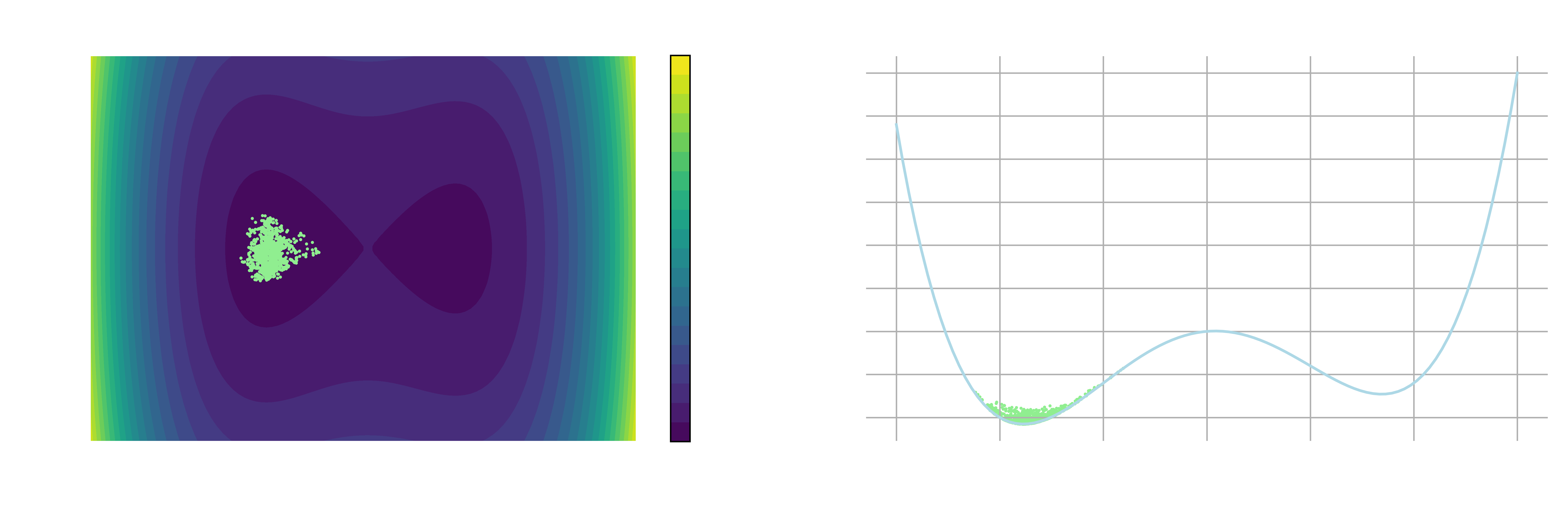
As supercomputing resources have become increasingly available in recent years¹, molecular dynamics (MD) has become a standard tool for studying atomistic-level behaviors of molecular systems in various scientific disciplines². However, an MD simulation can accurately describe the thermodynamic and structural properties of a system only if it achieves ergodicity during its simulation timescale. This means that the simulation must explore the phase space comprehensively, or equivalently, ensure that all possible configurations are sampled. This is usually a challenging task in real-world systems, as the metastable states of interest are frequently separated by substantial free energy barriers that are difficult to overcome by random fluctuations within a reasonable amount of time (see Figure 1 below, or the leftmost panel of Figure 1 in Chapter 2).

To overcome this limitation, researchers have developed various enhanced sampling methods in recent decades. One subset of these methods involves sampling along a set of predefined collective variables (CVs). These CVs, as we denote as a $d$-dimensional vector ${\bf \xi}=(\xi_{1}({\bf x}), \xi_2({\bf x}), …, \xi_d({\bf x}))$, can be any functions of the system coordinates ($\bf x$), such as torsions, coordination numbers, or radii of gyration. Ideally, CVs should represent a small number of degrees of freedom that capture the slowest degrees of freedom of the system and distinguish metastable states of interest. Some examples of CV-based methods include metadynamics, adaptive biasing force, umbrella sampling, and replica-exchange umbrella sampling, which will all be covered in this mini-course.

2. Terminologies

Before diving into the following chapters, we will review some key concepts in statistical mechanics by introducing a few terminologies one may come across in enhanced sampling methods. This section serves as a quick review of the essential concepts to better understand the tutorials in later chapters. Readers are encouraged to visit Section 2.2 (Glossary of essential notions) in the review by Hénin et al.³ for a more exhaustive list of terms.

Timescale

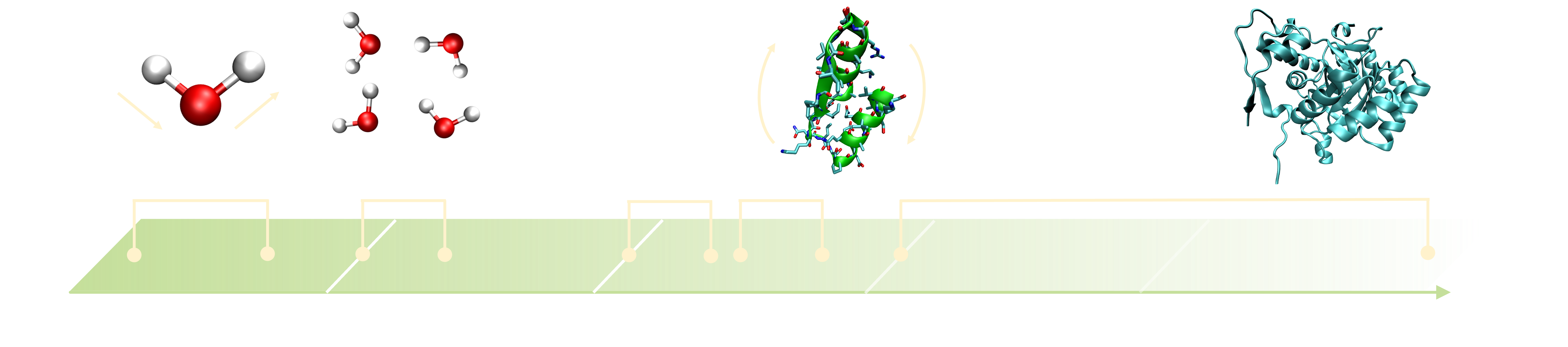
The real timescale of a molecular system can vary significantly depending on the size and complexity of the system, as well as the process of interest. As illustrated in Figure 2, the timescales of molecular motions can range from femtoseconds to seconds or even longer. For instance, bond vibrations, the fastest motion in a molecular system, typically occur on the order of femtoseconds. In contrast, biological processes such as allosteric transitions or protein-ligand binding have timescales considerably longer than bond vibrations, making the transitions between metastable states of interest rare events. This long timescale is due to the high free energy barriers separating metastable states, as discussed in the previous section.

Importantly, to ensure that the motion of atoms in a system is captured and no short-lived events are missed, such as bond vibrations and molecular rotations, the time step used in molecular dynamics simulations must be smaller than the shortest timescale in the system. This inevitably small time step makes simulations that study biological processes computationally expensive, easily requiring $10^8$ steps or more. To reduce the computational cost of simulating long-timescale processes, researchers frequently use enhanced sampling methods to bias the system towards the metastable states of interest. These methods make rare events more probable in a shorter timescale, thus reducing the number of required simulation steps.

Phase space and configuration space

In statistical mechanics, the phase space of a system is a space where all the possible states of the system can be represented. In three-dimensional Cartesian coordinate systems, a state is characterized by the coordinates ${\bf x} \in \mathbb{R}^{3N}$ and momenta ${\bf p} \in \mathbb{R}^{3N}$ of the system, where $N$ is the number of particles of the system. Consequently, each state can be represented by a unique point in the phase space, which is the joint space $({\bf x}, {\bf p})$.

In contrast, the configuration space is defined by all the possible configurations (defined solely by ${\bf x}$) of the system, so its dimensionality ($3N$) is half of that of the phase space ($6N$). When simulating long-timescale events using molecular dynamics, it is crucial to have sufficient sampling in the configuration space to capture the distribution of all possible configurations of the system. This ensures that rare events and transitions between different configurations are adequately represented. It is this need for comprehensive sampling in the configuration space motivates the development of enhanced sampling methods, which are the focus of this mini-course.

Microstate and macrostate

In the case where a system is composed of a larger number of particles, such as atoms or molecules, a microstate is a particular spatial arrangement of the particles in the system, i.e., a configuration. On the other hand, a macrostate, which can be defined by macroscopic thermodynamics variables (e.g., temperature, pressure, or total energy), is a collection of many possible microstates. For example, in a system composed of particles A and B that can either have an energy of 0 or 1, there are only three possible macrostates, which correspond to total energies of 0, 1, and 2, respectively. In the macrostate having a total energy of 2, there are two possible microstates: particles A and B having energies of 0 and 1, and the other way around.

Boltzmann distribution

To accurately calculate thermodynamic properties from molecular dynamics, we need to sample the Boltzmann distribution so that the system is at equilibrium. The Boltzmann distribution, sometimes called a Gibbs distribution, is a probability distribution that characterizes the distribution of states of a system in thermal equilibrium at a given temperature. It describes the probability of finding a particle in a particular energy state given its energy and the temperature of the system. Specifically, in the case where the energy levels are discrete, the normalized probability $p_i$ of finding the system being in state $i$ can be expressed as follows: $$\boxed{p_i = \frac{e^{-\beta E_i}}{\sum_i e^{-\beta E_i}} \propto e^{-\beta E_i}} \label{boltzmann_discrete} \tag{1}$$ where $E_i$ is the total energy (the sum of potential and kinetic energy) of state $i$, and $\beta = 1/k_{B}T$ is the inverse temperature (where $k_B$ is the Boltzmann constant ($1.38 \times 10^{-23} \text{ } \mathrm{J\cdot K^{-1}}$), and $T$ is the system temperature). Frequently, we denote the normalization constant as $Q=\sum_{i} e^{-\beta E_i}$, which is the so-called partition function.

In a phase space, where a state is defined by its continuous variables, coordinates ${\bf x}$ and momenta ${\bf p}$, we can rewrite the Boltzmann distribution as $$\boxed{\mu({\bf x}, {\bf p})=\frac{e^{-\beta(U({\bf x}) + K({\bf p}))}}{\int \int e^{-\beta(U({\bf x}) + K(\bf p))} d{\bf x}d{\bf p}} \propto e^{-\beta (U({\bf x}) + K({\bf p}))}} \label{boltzmann} \tag{2} $$ where $\mu({\bf x}, {\bf p})$, analogous to $p_i$ in the discrete space, is the probability of finding the system to have coordinates ${\bf x}$ and momenta ${\bf p}$. In this case, we have the partition function of the phase space $Q = \int \int e^{-\beta(U({\bf x}) + K(\bf p))} d{\bf x}d{\bf p}=\left ( \int e^{-\beta U({\bf x})}d{\bf x} \right ) \left (\int e^{-\beta K({\bf p})}d{\bf p} \right )$. Note that in Equation \ref{boltzmann}, we express the total energy as the sum of the potential energy $U({\bf x})$ and the kinetic energy $K({\bf p})$.

From Equation \ref{boltzmann}, we can derive the configurational distribution (the Boltzmann distribution in the configuration space) by integrating $\mu({\bf x}, {\bf p})$ with respect to the momenta ${\bf p}$: $$\nu({\bf x})=\int \mu({\bf x}, {\bf p}) d{\bf p}=\frac{1}{Q}\int e^{-\beta(U({\bf x})+K({\bf p}))}d {\bf p} = \frac{e^{-\beta U({\bf x})} \left ( \int e^{-\beta K({\bf p})}d{\bf p}\right )}{\left ( \int e^{-\beta U({\bf x})}d{\bf x} \right ) \left (\int e^{-\beta K({\bf p})}d{\bf p} \right )} \tag{3}$$ Finally, we have $$\boxed{\nu({\bf x})=\frac{e^{-\beta U({\bf x})}}{\int e^{-\beta U({\bf x})}d {\bf x}}\propto e^{-\beta U({\bf x})} \label{config_boltzmann}} \tag{4}$$ Frequently, Equation \ref{config_boltzmann} is written as $\nu({\bf x}) = \frac{1}{Z}e^{-\beta U({\bf x})}$, where $Z=\int e^{-\beta U({\bf x})}d{\bf x}$ is the configurational partition function.

Ensemble

In statistical mechanics, an ensemble is a collection of hypothetical copies of a system that all share the same macroscopic properties (such as temperature, pressure, volume, and chemical potential) but may differ in their microscopic details (such as the positions and velocities of individual particles). Some of the most common thermodynamic ensembles include

• NVT ensemble: The NVT ensemble is also called the canonical ensemble, where the number of particles ($N$), volume ($V$), and temperature ($T$) are fixed. The probability distribution and the corresponding partition function for the NVT ensemble are given by the Boltzmann distribution, namely, $$p_i = \frac{e^{-\beta E_i}}{\sum_i e^{-\beta E_i}}, \text{ } Z_{NVT} = \sum_i e^{-\beta E_i} \tag{5}$$
• NPT ensemble: The NPT ensemble is also called the isothermal-isobaric ensemble, or the Gibbs ensemble, where the number of particles ($N$), pressure($P$), and temperature ($T$) are fixed. The probability distribution and partition function of the NPT ensemble is given below: $$p_i = \frac{e^{-\beta E_i}e^{-\beta PV_i}}{\sum_i e^{-\beta E_i}e^{-\beta PV_i}}, \text{ } Z_{NPT} = \sum_i e^{-\beta E_i}e^{-\beta PV_i} \tag{6}$$
• NVE ensemble: The NVE ensemble is also called the microcanonical ensemble. The NVE ensemble is defined by assigning an equal probability to every microstate whose energy falls within a range centered at $E$, and all the other microstates are given a probability of 0. That is, the probability in the NVE ensemble can be written as $p_i = 1/W$, where $W$ is the number of microstates within the range of energy.
• $\mu$VT ensemble: The $\mu$VT ensemble is also called the grand canonical ensemble, where the chemical potential ($\mu$), volume ($V$) and temperature ($T$) are fixed. The probability distribution and partition function of the $\mu VT$ ensemble is given below: $$p_i = \frac{e^{-\beta E_i}e^{\beta \mu N_i}}{\sum_i e^{-\beta E_i}e^{\beta \mu N_i}}, \text{ } Z_{\mu VT} = \sum_i e^{-\beta E_i}e^{\beta \mu N_i} \tag{7}$$

Notably, given the copies of the system in an ensemble, we can calculate the ensemble average of an observable $O({\bf x}, {\bf p})$ of interest, which is simply taking the average of $O({\bf x}, {\bf p})$ considering all points $({\bf x}, {\bf p})$ in the phase space: $$\langle O \rangle = \int O({\bf x}, {\bf p})\mu({\bf x}, {\bf p})d{\bf x}d{\bf p} \tag{8}$$

Ergodicity

The dynamics of a system is said to be ergodic if the ensemble average of the observable $O({\bf x}, {\bf p})$ of interest is equal to the time average of the observable over an infinitely long trajectory, namely, $$\langle O \rangle = \int O({\bf x}, {\bf p})\mu({\bf x}, {\bf p})d{\bf x}d{\bf p} = \lim_{M\rightarrow \infty} \sum_{t=1}^M O({\bf x}_t, {\bf p}_t) \tag{9}$$ In simple terms, if one monitors an obervable of interest for a single particle over a sufficiently long period of time and take the average of the observable at all time frames, the outcome would be equivalent to the average of the same observable computed over all possible configurations of the system at a single instant. In practice, given that it is impractical to identify all possible configurations at any given time frame, reaching ergodicity in molecular dynamics is essential as it allows one to estimate the ensemble average by computing the time average over a sufficiently long trajectory.

Metastable state

Metastable states are the states having a higher potential energy than the ground state but are stable enough for the system to reside for an extended (but finite) amount of time. For example, there are two metastable states in Figure 1. One has values of $x_2$ around -1.8, while the other has values of $x_2$ around 1.8.

Collective variable (CV)

Here, we refer to collective variables (CVs) as a $d$-dimensional vector ${\bf \xi}=(\xi_{1}({\bf x}), \xi_2({\bf x}), …, \xi_d({\bf x}))$, which can be seen as a lower-dimensional representation reduced/projected from the full $3N$-dimensional configurations ${\bf x}$ via the mapping function $\Phi({\bf x})={\bf \xi}$, with $d \ll 3N$. Traditionally, CVs can be defined as any functions of the coordinates of the system, but could additionally include the alchemical variable, as shown in a recent paper proposing alchemical metadynamics⁴, the method we will explore in Chapter 7.

Ideally, an optimal set of CVs should be able to capture the slowest dynamics of the system and distinguish the metastable states of interest. For example, in Figure 1, $x_1$ is a reliable CV for distinguishing the two metastable states of interest. Conversely, $x_2$ is orthogonal to the slowest degree of freedom of the system and, therefore, is not suitable for describing transitions between the two metastable states. Identifying the optimal set of CVs is often challenging in systems where the slowest-relaxing coordinates are not intuitive. In such cases, machine learning-based algorithms like RAVE⁵ or SGOOP⁶ can be helpful.

Free energy

In the canonical (NVT) ensemble, Helmholtz free energy is defined as $$F=-\frac{1}{\beta}\ln Z_{NVT}=-\frac{1}{\beta}\int e^{-\beta U({\bf x})}d{\bf x}\tag{10}$$ while in the Gibbs (NPT) ensemble, the Gibbs free energy can be expessed as $$G=F+PV=-\frac{1}{\beta}\left[ \ln Z_{NVT} - \left( \frac{\partial \ln Z_{NVT}}{\partial \ln V} \right )\right] \tag{11}$$ Practically, in a soluted system where the solvent is nearly imcompressible, i.e., $\frac{\partial V}{\partial P}\approx 0$, the difference in Gibbs free energy is almost equal to the difference in Helmholtz free energy.

Free energy profile

A free energy profile is meaningful only if there is a collective variable ${\bf \xi}$ of interest. A free energy profile, sometimes called a free energy landscape or a free energy surface, can be computed as follows: $$\boxed{F({\bf \xi})=-\frac{1}{\beta}\ln P({\bf \xi}) = -\frac{1}{\beta}\ln \int \delta({\bf \xi} - \Phi({\bf x}))\nu({\bf x})d{\bf x}=-\frac{1}{\beta}\langle \delta({\bf \xi}-{\bf \xi}({\bf x}))\rangle} \label{free_energy}\tag{12}$$ where $\nu({\bf x})=e^{-\beta U({\bf x})}/\int e^{-\beta U({\bf x})} d{\bf x}$ is the Boltzmann distribution and $\Phi$ is a function mapping the $3N$-dimensional vector ${\bf x}$ to the $d$-dimensional CV vector ${\bf \xi}$. The function $\delta$ is the multivariate Dirac delta function, i.e., $$\delta({\bf \xi}-\Phi({\bf x}))=\prod_i^d \delta'(\xi_i-\Phi_i({\bf x})), \text{ } \delta'(\xi_i-\Phi_i({\bf x}))=\begin{cases}+\infty \text{, if } \xi_i=\Phi_i({\bf x})\\ 0 \text{, otherwise} \end{cases}\tag{13}\label{delta}$$ where $\delta’$ is a single-variable Dirac delta function and $\Phi_i$ is a function mapping ${\bf x}$ to the $i$-th CV, $\xi_i$. While Equations \ref{free_energy} and \ref{delta} may seem daunting, they essentially mean that the free energy profile along the CVs can be computed from the marginal probability density $P({\bf x})$ along the CVs, which is obtained by integrating the Boltzmann distribution $\nu({\bf x})$ over all variables except for the CVs $\Phi({\bf x})$. This interpretation may be understood more easily with the example in the Supplementary note below.

Free energy estimator

A free energy estimator is an expression or algorithm that is used to estimate free energy differences or free energy surfaces from simulation data, such as configurations, energies, and forces. Other than estimating free energy by directly measuring the probability ratios or from transition matrices, common free energy estimators include weighted histogram analysis method (WHAM)⁷, thermodynamic integration (TI)⁸, Bennett acceptance ratio (BAR)⁹, and multistate Bennett acceptance ratio (MBAR)¹⁰. These free energy estimators will be briefly introduced in the following chapters.

Potential of mean force (PMF)

While the term potential of mean force (PMF) is frequently used interchangeably with free energy surface, the historical definition of PMF is defined between two particles 1 and 2 and represents the effective potential energy that particle 1 experiences due to the presence of particle 2, when the positions of all other particles in the system are averaged over. It is defined based on the radial distribution function $g(r)$: $$\boxed{W(r)=-\frac{1}{\beta}\ln g(r) = F(r) + \frac{2}{\beta} \ln r + C} \tag{14}$$ where $F(r)$ is the free energy surface along the interparticle distance and $C$ is an arbitrary constant. That is, the historic definition of PMF is related to the free energy surface but is still a distinct quantity. Check the Supplementary note below to see how PMF relates to the radial distribution function. In this mini-course, we treat the term “potential of mean force” equivalently as the term “free energy profile”.

3. Exercises

👨‍💻 Exercise 1

Given the functional form of the free energy surface in Figure 1 ($f(x_1, x_2)=x_1^4-6x_1^2+x_1+x_2^2$), estimate the timescale of transitioning from the left to right metastable states at 300 K. (Hint: One can use the transition state theory (TST) to estimate the rate constant of the process.)

👨‍💻 Exercise 2

A one-dimensional simple harmonic potential with a force constant $K$ can be expressed as $U(x)=\frac{1}{2}K(x-x_0)^2$, where $x_0$ is the equilibrium position on the $x$-axis. Given this, derive the probability density distribution and Helmholtz free energy expressions for the system.